
Mass screening is an essential element in the fight to curb the spread of coronavirus. But how can a possible shortage of reagents and equipment be avoided? By testing mixtures of samples and relying on mathematics.
With the anticipated fear of a second wave of COVID-19, many experts agree that large-scale screening is necessary to stop the spread of coronavirus. Immunological, serological or antigenic testing of representative samples from the population can also help to estimate the prevalence of the disease, assess herd immunity and adapt pandemic management measures.
Successful implementation of a mass screening strategy requires access to substantial resources in terms of personnel and equipment. With increasing global demand, a shortage of reagents needed for laboratory testing has rapidly emerged on the horizon and remains a concern for public health authorities in Canada and around the world.
Given that, for the most part, the tests are (fortunately) negative, can we use mathematics to do better? It turns out that yes, notably by carrying out group tests on judiciously constructed mixtures of samples.
Group screening
Suppose that a laboratory has received 100 samples for diagnostic testing. It randomly divides them into 5 groups of size 20. Then, group by group, it uses half of each of the 20 samples to make a mixture and applies the test to it.
If a test on a pooled sample is negative, it can be immediately concluded that no one in the pool is infected. If the test is positive, then the second half of each of the 20 samples is tested individually.
If the initial 100 samples come from healthy individuals, this procedure reduces the number of tests to be performed from 100 to 5. If only one individual is infected, then 5 + 20 = 25 tests are sufficient to identify that person. If two individuals are infected, 25 tests are also sufficient to identify them if they are in the same group but 5 + 20 + 20 = 45 tests are needed if they belong to different groups. And so on if there are three or more infected people.
As can be seen, group screening can translate into significant savings, provided of course that the sensitivity and specificity of the test are not affected by mixing, as has been assumed above since this is very often the case in practice.
Alternatively, the laboratory could have applied the same screening strategy to 10 groups of 10 samples. If only one individual is infected, then only 20 tests are needed to identify that person. However, it then takes 10 tests to conclude that no one was infected.
Which of these two strategies is better? And are there others that are preferable? The answer depends on the prevalence of the disease, i.e., the proportion of the population that is infected.
In a 1943 note published in The Annals of Mathematical Statistics, Robert Dorfman reported that, in its most basic form, group screening had already been used during World War II to test US army drafts for syphilis. The approach became the standard and there are now many variations of this approach, including testing throughout North America for HIV, influenza and West Nile Virus.
Optimizing the algorithm
Dorfman showed how to determine the optimal group size based on the $p \in [0, 1]$ prevalence of disease. Denote by $n ≥ 2$ the size of the group and assume that its members form a random sample which is representative of the population.
If $X$ denotes the unknown number of infected persons in the group, then this variable follows a binomial distribution 1 with parameters $n$ and $p$, from which
\[\text{Pr}(X=0)=(1–p)^n,\]
since each individual has a probability $1-p$ of being healthy, and
\[\text{Pr}(X>0)=1–\text{Pr}(X=0)=1–(1–p)^n.\]
If $X=0$, then one only needs to perform $N =1$ test. However if $X >0$, then $N=n+1$ tests will be needed. The average number of tests to be performed, called expectation of $N$ and noted $E(N)$, is equal to
\[\begin{array}{r c l}E(N) &=&1×\text{Pr}(X=0)+(n+1)×\text{Pr}(X>0) \\&=& n+1-n(1-p)^n.\end{array}\]
This function is increasing in $p$. If $p = 0$ we have $E(N) = 1$, which is obvious since nobody has the disease and therefore a single test is needed to confirm it. If $p=1$, we have $E(N)=n+1$ because the first test will necessarily be positive.
For any value of $p \in [0, 1]$, it is possible to determine the relative cost related to the use of group screening by studying the behaviour of the ratio
\[E(N)/n=1+1/n–(1–p)^n\]
as a function of $n$. The smaller $E(N)/n$ is, the more it pays to use group testing, provided of course that the ratio is less than $1$. When $p = 0$ we find $E(N)/n=1/n$, so it pays to take $n$ as large as possible. When $p = 1$, we always have
\[E(N)/n=1+1/n>1\]
because the group test is always positive and therefore only adds to the burden.

Figure 1
Plot of the curve $100×E(N)/n$ versus $n$ for different values of p: 1% (black), 2% (brown), 5% (orange), 8% (red), 10% (blue) and 15% (green).
For a fixed value of $p$, the function $100 \times E(N)/n$ represents the average percentage of tests performed as a function of the size, $n$, of the group. The figure shows the graph of this function for different values of $p$, corresponding to a prevalence of 1% (black), 2% (brown), 5% (orange), 8% (red), 10% (blue) and 15% (green). As can be seen, the optimal size of the mixtures, which corresponds to the minimum of the curve, varies according to the proportion, $p$, of infected individuals in the population. The table below, reported by Dorfman, gives the optimal choice of $n$ for a few values of $p$.
| $p$ (%) | $n$ | Relative cost (%) |
| 1 | 11 | 20 |
| 2 | 8 | 27 |
| 5 | 5 | 43 |
| 8 | 4 | 53 |
| 10 | 4 | 59 |
| 15 | 3 | 72 |
Generalizations
The testing protocol described above is an example of a two-round adaptive algorithm. It is said to be adaptive because the choice (and therefore the number) of tests to be performed in the second round depends on the result of the test performed in the first round. There are several ways to improve the performance of this type of algorithm. In particular, the procedure can be extended by increasing the number of rounds.
Here is a classical algorithm, which we will call binary division algorithm, and which has certain optimality properties (see Figure 2).
a) Take an integer $n$ of the form $n = 2^s$ and perform $k$ rounds of tests, where $k ≤s+1$.
b) In the first round, test a mixture of samples from the whole group.
c) If the test is positive, then the group is divided into two subgroups of $2^{s-1}$ samples and a mixture of each is tested.
d) This is continued until the $k$th round, where all members of a subgroup that was positive in the previous round are tested individually. In the particular case $k=s+1$, this subgroup has only two items left.

Figure 2
Graphical representation of an adaptive 5-round binary division algorithm applied to an initial sample of $n = 2^4 = 16$ individuals, only one of whom is infected.
If the group contains a single infected individual, this algorithm will identify him/her in exactly $s+1=\log_2(n)+1$ rounds. As a general rule, the higher the number of rounds, the better the savings generated by this approach. However, if it takes 24 to 48 hours for a test to be conclusive, the turnaround time for delivery of analysis results may be counterproductive. It should also be noted that this improvement requires larger biological samples. This is not really considered a problem and will be assumed in all the algorithms presented below.
A non-adaptive algorithm
To better control response time, non-adaptive group screening methods may also be considered. These protocols involve only one round, allowing all tests to be performed simultaneously. They are very effective for case detection if a reliable estimate of the prevalence of the disease is available.
Let’s explain the concept using the following example, developed by a team of Rwandan researchers as part of the current COVID-19 response. First, a random sample of size $n = 3^m$ is drawn. Next, a correspondence is established between the $3^m$ individuals and the points of a discrete hypercube $\{0, 1, 2\}^m$. See Figure 3 for an illustration in the case $m = 3$.
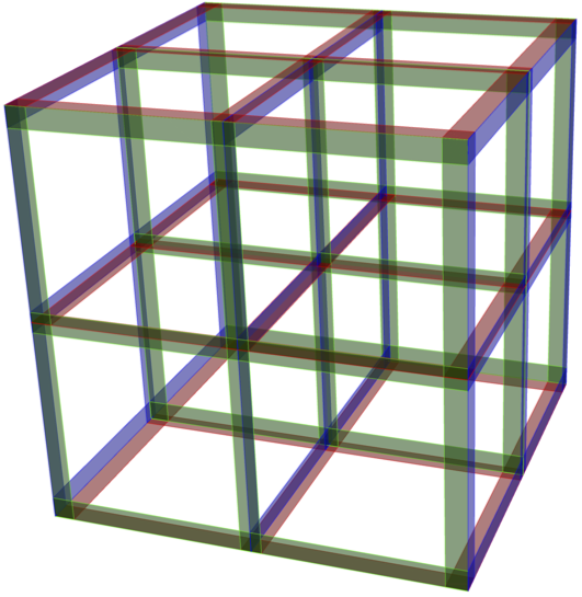
Figure 3
Discrete hypercube $\{0,1,2\}^3$. Each point of the lattice corresponds to an individual in a random sample of size $n=3^3=27$. The $3^2=9$ individuals forming each of the 9 mixtures are located along a red, blue or green slice.
The proposed approach then consists in simultaneously performing $3m$ tests on mixtures of samples each containing $3^{m-1}$ individuals. However, the pools are made up according to very specific modalities, i.e., slices of the hypercube. Indeed, if $x_1,\ldots,x_m $ denote the coordinate axes of the hypercube, each of the mixtures corresponds to the individuals located in the hyperplane $x_i=t$, where $i\in \{1,\ldots,m\}$ and $t\in \{0,1,2\}$ is a slice of $3^{m-1}$ individuals.
When $m = 3$ as in Figure 3, then $3 \times 3 = 9$ tests are performed on groups of $3^2 = 9$ individuals. When $m = 4$, which is the value used for the implementation in Rwanda, 12 tests are performed on a random sample of $n = 81$ individuals. This means that each sample is divided into four equal portions and contributes to four different tests. In addition, each test is a mixture of 27 samples.
This approach is based on an error-correcting code construction technique described in the box. One of its great advantages is that the composition of the mixtures is such that if there is only one infected individual in the sample, he or she can be identified with certainty. If more than one person is infected, however, then a second round of testing is required.
Let us examine the Rwandan example in the case $n = 81=3^4$. Knowing that the number $X$ of infected individuals in the sample follows a binomial law with parameters $n = 81$ and $p$, we have
\[\text{Pr}(X ≤1)=(1 – p)^{81}+81p(1-p)^{80}.\]
This strategy is interesting if the probability that $X ≤ 1$ is large. But to ensure that $\text{Pr}(X ≤ 1) ≥ 0.95$, for example, one must have $p ≤ 0.44\%$; in other words, the prevalence of the disease must be low. Already, at 1% prevalence we have $\text{Pr}(X ≤ 1) = 0.806$ and in almost 20% of cases we will have to resort to a second round. However, still for 1% prevalence, we have
\[\text{Pr}(X=2)=\pmatrix{81 \\\ 2}p^2(1-p)^{79}=0.146,\]
hence $\text{Pr}(X ≤ 2) = 0.952$.
Costs can easily be controlled if we are clever in the way we conduct the second round when there is more than one infected individual. For example, all cases corresponding to $X =2$ satisfy the following property (refer to Figure 4 where we show, in the case of $m = 3$, the brackets with a positive test):
(P) For any value of $i \in \{1, \ldots, m \},$ there are at most two slices of the form $x_i = s$ and $x_i = t$ leading to a positive test, and there is at least one value of $i$ for which there are exactly two such slices leading to positive tests.

Figure 4
The discrete hypercube $\{0, 1, 2\}^3$ and the three possibilities for two infected individuals: on the same straight line parallel to an axis (left), at opposite vertices of a square in a plane (center) or at opposite vertices of a cube (right). In each case, the slices leading to a positive test are identified in red, green or blue with the same color conventions as in Figure 3.
If $k$ is the number of values of $i \in \{ 1,\ldots ,m \}$ for which there are two positive tests of the form specified in (P), the number of additional tests required to identify all infected individuals is given in the following table.
| $k$ | Number of additional tests |
| 1 | 0 |
| 2 | 4 |
| 3 | 8 |
| 4 | 16 |
If property (P) does not hold, then all individuals in the slices that test positive must be tested, resulting in a maximum of 81 additional tests. In the end, the total relative cost turns out to be equal to 100 × 17/81 ≈ 21%.
Perspectives
The search for algorithms adapted to the fight against the coronavirus is in full swing. For example, an algorithm was recently developed and implemented in a laboratory by an Israeli research team. It consists of performing 48 tests on a single random sample of size $8 \times 48 = 384$, with each individual sample divided into six equal parts. Each of the tests is based on the mixture of 48 of these shares, one per individual. Each individual’s sample is therefore present in six different tests. In the laboratory, a robot has been programmed to prepare the 48 mixtures. The algorithm can identify up to four infected individuals. This means that eight times fewer tests are needed than individuals. Again, the smaller the percentage of infected individuals, the better the performance of the algorithm.
Of course, other considerations come into play when developing a statistical testing procedure. For simplicity, we have implicitly assumed here that the test used is infallible. In practice, even the best procedures can give false positives or false negatives. The sensitivity and specificity of a test are important considerations when recommending its implementation, as well as its feasibility in terms of time, cost and manipulations.
Building a non-adaptive algorithm
We want to build a non-adaptive algorithm to test a group of people. We will represent this algorithm by a table with $T$ rows and $n$ columns, or equivalently by a matrix of dimension $T × n$ all of whose entries are equal to $0$ or $1$. The $i$th row of the matrix corresponds to the $i$th test. The entries equal to $1$ in the $j$th column represent the tests in which the $j$th individual is involved. Thus, $m_{ij} = 1$ if the $j$th individual contributes to the $i$th test and $m_{ij} = 0$ otherwise.
Let’s construct a vector $X$ of length $n$ representing the group to be tested: its $i$th coordinate, $x_i$, is $1$ if the $i$th individual is infected and $0$ otherwise. We treat $X$ as a word of length $n$ and its few coordinates equal to $1$ as errors in the transmission of the word $X_0$ whose coordinates were all equal to zero originally. Error-correcting code algorithms are used to correct the errors that have occurred in the transmission of $X_0$, which amounts to identifying the coordinates $x_i$ of $X$ that are equal to $1$, which is exactly the intended purpose. In general, an error correction algorithm can only correct at most $k$ errors, where the value of $k$ is predetermined.
The matrix $M$ is the matrix of the code. A sufficient property for the code to correct $k$ errors is that this matrix be $k$-disjoint. Let’s define this notion. We want to avoid that a $j_{k+1}$th infected individual goes unnoticed when individuals $j_1, \ldots, j_k$ (not necessarily distinct) are infected. There is a one-to-one correspondence between column $j$ (i.e., individual $j$) and the set $A_j$ of elements of $\{1, \ldots , T\}$ corresponding to entries equal to 1 (i.e., the set of tests to which in which individual $j$ is involved). If individuals $j_1, \ldots, j_k$ are infected, then all tests corresponding to the set $A_{j_1} \cup \cdots \cup A_{j_k}$ will be positive. In order for the $j_{k+1}$th infected individual not to go unnoticed, the set $A_{j_{k +1}}$ must not be a subset of $A_{j_1} \cup \cdots \cup A_{j_k}$. The matrix $M$ is $k$-disjoint if this is the case for all $j_1, \ldots , j_k$ and any $j_{k+1}$ distinct from $j_1, \ldots, j_k$. The $12 \times 81$ matrix corresponding to the above example used in Rwanda is a 1-disjoint matrix.
There are two main strategies for constructing $k$-disjoint matrices. The first is probabilistic: matrices are randomly generated with entries equal to $1$ with probability $q$ and $0$ with probability $1-q$. For suitably chosen values of $n$, $T$ and $k$, the probability that the matrix is $k$-disjoint is non-zero; a $k$-disjoint matrix can thus be generated by trial and error.
The second method, which is algebraic, stems from the Reed-Solomon error-correcting code theory. It makes it possible to build matrices $M$ in which all rows have the same number $m$ of non-zero entries and all columns have the same number $c$ of non-zero entries. Accordingly, all the tests are done on subgroups of size $m$ and each individual contributes to $c$ separate tests.
- This approximation is reasonable provided that the population is large in relation to the size of the groups ↩